Diwali has just passed and the festivities are dialling down. Diwali has brought changes for Telerik in India and now I write this as an evangelist for Telerik/ Progress. In this blog post, I will list the changes and attempt to clarify if it has any impact on our community:
Telerik (a part of Progress) has changed its operations structurally in India. Indian Rupee billing was number one request from businesses who found USD billing to a US entity time taking and troublesome.
Telerik products will now be sold in India in Indian Rupees only via a distributor.While this does not affect you as a developer, your accounts team and business managers would love this change due to the following:
A lot less hassle in making the payments done. Earlier, they had to get multiple forms (Form 15 CA & Form 15 CB) signed from a Chartered Accounts and make the payment via a wire transfer through the bank. This could take over 4-5 days to make a single payment and accrue additional charges for the wire transfer. Now, it is a simple NEFT or a UPI transfer.
Lowering cost of projects to the customers. Earlier products like Telerik DevCraft couldn’t be used to offset indirect tax liability. With the new GST regime, your accounts team can offset the tax on their project lowering the cost of the implementation for their customers in India.
Isn’t this just great?
The new distributor is GTM Catalyst for the India market. What is even better is that I will be handling this new distributor organisation. This will bring the familiarity and continuity of business for you.
You may reach GTM Catalyst team for any questions or comments at: info@gtmcatalyst.com
To allay any questions in your mind, all the Telerik products continue to be available for sales and are fully supported by Telerik/ Progress. All products are moving full steam ahead including DevCraft, Kendo UI, Telerik Platform, Telerik Reporting, Sitefinity and Test Studio. Telerik (a Progress company) will continue to release new updates on a rigorous pace and continue to provide you with benefits of the latest technologies.
Lastly, we are eager to continue our India webinar series to share our learnings with you. We will be sending the webinar schedule to you shortly with an update here.
Generative AI (GenAI) tools — from ChatGPT and Gemini to Claude — are no longer just innovation experiments. They’re embedded in workflows, customer journeys, and enterprise applications.
But with that opportunity comes a sharp reality: GenAI introduces new data privacy risks that most corporate systems were never designed to handle.
This article breaks down:
The top privacy challenges organisations face when adopting GenAI.
What enterprise-grade solutions offer to mitigate these risks.
Practical steps for enterprises and project managers to operationalise GenAI safely.
Why Privacy Matters More Than Ever
GenAI thrives on data — but that’s exactly where its risk lies. Every prompt, document, or snippet entered could become a data-governance concern.
The Core Privacy Risks
Risk
What It Means
Why It Matters
Data Leakage & Unintended Exposure
Employees may paste sensitive (PII) or proprietary data into public GenAI tools, losing control once it leaves the org boundary.
Studies (Deloitte) show 75% of tech professionals rank privacy as a top GenAI concern.
Unintended Model Training
Non-enterprise versions may use user inputs for model improvement.
Proprietary IP could be absorbed into shared models.
Ownership & Retention Ambiguity
Consumer tools often lack clarity on who owns prompts and outputs or how long data is stored.
Creates legal uncertainty around IP and auditability.
Regulatory Compliance Gaps
GenAI usage must align with GDPR, CCPA, and emerging AI Acts.
Non-compliance risks penalties and reputation loss.
Shadow IT & Unapproved Usage
Employees may use personal GenAI accounts.
Creates blind spots for data exposure and audit gaps.
Bottom Line: GenAI amplifies traditional data risks — because the data flows are richer, models more opaque, and control boundaries blur faster.
The Solution: What It Looks Like
The solution lies in ensuring that GenAI tools respect the data privacy of the documents uploaded. The way GenAI tools have struck a balance is to offer “privacy” as a feature in their enterprise editions.
When enterprises upgrade to enterprise editions of GenAI tools, they gain visibility, ownership, and control. Let’s examine OpenAI’s enterprise commitments as an example blueprint.
1. Ownership & Control of Data
“You own and control your data. We do not train our models on your business data by default.” — OpenAI Enterprise Privacy
✅ Inputs and outputs remain your property. ✅ You control data retention. ✅ No auto-training on business data.
Why it matters: Enterprises retain IP rights, reduce legal ambiguity, and align with data-minimisation and right-to-erasure principles.
2. Fine-Grained Access & Authentication
SAML-based SSO integration
Admin dashboards to control who can access what
Connector governance to approve or restrict data sources
Why it matters: Access governance limits who can interact with sensitive data — and how. Permissions reduce accidental or malicious data exfiltration.
3. Security, Compliance & Certifications
AES-256 encryption at rest; TLS 1.2+ in transit
SOC 2 Type II certification
BAA & DPA support for regulated sectors (e.g., healthcare, finance)
Why it matters: Aligns GenAI use with enterprise IT standards and compliance requirements.
4. Data Retention & Deletion Controls
“Admins control retention. Deleted conversations are removed within 30 days.” — OpenAI
Zero-Data-Retention (ZDR) for API endpoints
Custom deletion timelines
Why it matters: Enables compliance with right-to-erasure laws and reduces long-term data exposure risk.
5. Model Training & Fine-Tuning Controls
No business data used for training without explicit opt-in.
Fine-tuned models remain exclusive to the enterprise.
Why it matters: Prevents proprietary data from bleeding into shared models. Protects confidential business logic and datasets.
Translating Commitments into Enterprise Practice
Here’s how to operationalise privacy-by-design in your GenAI strategy.
Step
Action
Why It Matters
1
Create a “What Goes into GenAI” Policy
Ban sensitive data (PII, source code, contracts) unless approved.
2
Use Enterprise Licenses
Ensure tools provide encryption, retention control, and no auto-training.
3
Govern Connectors
Limit which internal systems feed into GenAI tools.
4
Define Retention Rules
Configure retention periods and deletion workflows.
5
Monitor Usage
Use compliance APIs to track prompts, access logs, and connectors.
6
Train Employees
Reinforce responsible usage and red-flag categories (finance, HR, IP).
7
Align with Legal & Governance Policies
Map GenAI practices to your data-governance framework and DPIAs.
8
Use ZDR Endpoints for Sensitive Data
Required for regulated or confidential workloads.
9
Review Regularly
Re-audit tools and contracts as regulations evolve.
Applying It to Your Context: ERP & Project Management
For ERP implementations — where financial, HR, and vendor data converge — the stakes are higher.
Data boundaries: Never use GenAI with live financial or payroll data unless the endpoint is enterprise-secured.
Vendor contracts: Ensure client or third-party NDAs don’t prohibit AI-based processing. Include a section that mentions that contracts may be reviewed by GenAI tools.
Governance embedding: Add GenAI checkpoints in your project governance map — who approves prompts, what is logged, how outputs are validated.
Model isolation: When fine-tuning internal GenAI workflows, use isolated models to prevent cross-project exposure.
The Takeaway
Generative AI unlocks speed and scale, but data privacy is the cost of entry for responsible adoption.
Enterprise GenAI tools — like OpenAI’s ChatGPT Enterprise — now offer the controls and transparency needed for compliant, secure innovation. Yet, technology alone isn’t enough.
Enterprises must also embed:
Governance (policies & audits)
Awareness (training & culture)
Alignment (legal & regulatory frameworks)
For project managers and IT leaders, the mission is clear: 👉 Innovate boldly, govern responsibly, and ensure that data privacy remains the cornerstone of your GenAI strategy.
We recently had a case where a customer was running Azure Databricks notebook from Azure Data Factory. They mentioned that the configuration used to run the notebook was not secure as it was associated with a user account (probably a service account). The username and password was known to multitude of users and it had already caused some trouble. The concept of a “service account” has been quite prevalent since the times of on-premise applications. The service account was a user account that was used to run various applications and nothing else. In the modern world of cloud services, service accounts are obsolete and should never be used.
He wondered if there was a better way to run such notebooks in a more secure way?
In a single line, the solution to this problem is running the notebook as a service principal (and not a service account).
Here is a detailed step by step guide on how to make this work for Azure Databricks notebooks running from Azure Data Factory:
Generate a new Service Principal (SP) in Azure Entra ID and create a client secret
Add this Service Principal to the Databricks workspace and grant “Cluster Creation” rights
Grant this Service Principal User Access to the Databricks workspace as a user
Generate a Databricks PAT for this Service Principal
Create a new Linked Service in ADF using Access Token credentials of the Service Principal
Create a new workflow and execute it
If you followed the above instructions, your Databricks notebook will be run as a Service Principal.
One thing to understand before going over the detailed steps is the fact that when you add a Databricks notebook as an activity in Azure Data Factory, you are creating an “ephemeral job” in Databricks in the background when the ADF pipeline is run. You can control what kind of job cluster gets created and the user credentials under which the job will be run based on the linked service settings. Let’s get started:
Generate a new SP with client secret
Go to portal.azure.com and search for “Microsoft Entra ID” in the search tab and click it
Click on Add and select “App registration”
Give a meaningful name and leave the rest as-is and click “register”
You should now see something like below
Now click on “Certificates & secrets” and under the “Client secrets” tab click “New client secret”
Under the “Add a client secret” pop-up, give a meaningful description and choose the appropriate expiration window and click “create”. Once done you should see something like this under the “Client secrets” tab
Now open a notepad and have all the information noted there. Host: Databricks workspace URL Azure_tenant_id and Azure_client_id will be what is shown in the image under point 4 Azure_client_secret will be the value in the image under point 6
2. Add this Service Principal to the Databricks workspace and grant “Cluster Creation” rights
Now go to your target workspace and click on your Name to expand the menu, click open the settings( this requires workspace admin privilege)
Now click on” identity and access” and under service principals click on manage
Click on “add service principal” button Now click on Add new Select the “Microsoft Entra ID managed” radio button and populate with the Application ID(client id) and give the same name as shown in point 4 and click Add Now provide “Allow cluster creation” permission to the service principal to ensure it can create a new job cluster when we run through an ADF and click “update”
Generate a Databricks PAT for this Service Principal
If you are on Mac open the terminal and use the command “nano .databrickscfg” to open the databricks config file and paste the information from the notepad from point 8. If you are on Windows press windows + R and type “notepad %APPDATA%\databricks\databricks.cfg” and press enter. Now paste the information from the notepad from point 8 into the Databricks config file. You will also have to give a meaningful profile name to identify the workspace in the config file.
The config file should look like below once you are done. [hdfc-dbx] is the profile name here.Save and exit.
Now go to Databricks CLI and authenticate the service principal’s profile using a PAT token by typing “databricks configure”. It will prompt for the host workspace’s URL and PAT token, provide it, and press enter.
Now goto databricks cli and generate a PAT token for the Service Principal using the command “databricks tokens create –lifetime-seconds 86400 -p <profile name>”. You should see a proper response like below:
Now grab the “token value” and keep it in a notepad safely
Create a new Linked Service in ADF using Access Token credentials of the Service Principal
Now go to ADF, click on Manage -> Linked services -> New Under New Linked Service popup click on “compute” and select “Azure Databricks” click continue
Now provide a meaningful name to the linked service, select the proper Azure subscription, and your target workspace. Under Authentication Type leave the option as Access Token and under the access token field update the access token we generated in point 13.(This is being done as an interim solution, the best practice is to use an Azure Key Vault and pass the token through secret).
Now select the cluster version as 13.3 LTS, Node type, Python version, and Worker options as relevant to current cluster configuration. You can select the UC Catalog Access Mode as “Assigned” for single user and “Shared” for shared access mode. Click on test connection to ensure everything is working as intended.
Create a new workflow and execute it
Now create a pipeline select the linked service that you created and point the ADF to a notebook.
Click “Debug” and the job should run successfully
If you open the job execution link, you can see the job has been run as a Service Principal under task details
This is indicated by the value against “Run as” which is that of the Service Principal.
The Indian government has recently passed the Digital Personal Data Protection Bill (DPDP) in 2023. This is a significant step towards establishing a framework for managing citizens’ data in India.
Previously, data protection was governed by the Information Technology Act of 2000 (Section 21). With this law, customers have been granted specific rights over their data including correction, erasure, grievance redressal, and withdrawing consent.
For every marketer in India, it’s essential to understand and follow the provisions of the DPDP law to avoid severe penalties. Whether you do digital marketing, events marketing or are an organisation collecting data, this bill affects you. Even companies collecting data from their employees are within ambit of this law.
Penalties for Data Fiduciaries/ data collectors breaching customer data security can reach up to Rs 250 crore or USD 30 mn. Penalties are influenced by severity, repetition, and actions taken by the fiduciary.
In this blog post, we’ll highlight the key points of this law that are relevant for marketers:
To grasp the DPDP, it’s important to know the main entities involved:
Data Fiduciaries: These are the parties primarily responsible for handling data. As a website owner, you are a Data Fiduciary.
Data Principals: These are your customers or individuals whose data you are handling.
Data Processors: These are entities that process data on behalf of Data Fiduciaries. Processing includes various operations like collecting, storing, transmitting, and more.
Whether your website is hosted in India or abroad, if it deals with data of Indian citizens, the DPDP law applies (Section 3(b)). As website owners, you can appoint a different Data Processor (Section 8(2)), but you are responsible for data handling and ensuring the processor complies by implementing appropriate measures. This means that you can use external service providers e.g. for emails, SMSs, Whatsapp, Social Media but are responsible for their adherence to these laws.
Obligations of Data Fiduciaries are as follows:
Processing for Lawful Purposes (Section 4): Data can only be used for lawful purposes for which the data principal has given consent. You need to notify individuals about the purpose of data collection at the time of data collection. If you acquired customers before this law was enacted, you must provide this notification as soon as possible. The burden of proof for consent lies with the Data Fiduciary.
Consent and Withdrawal (Section 6): Individuals can withdraw consent at any time, and you must stop processing their data within a reasonable time (not defined). This includes deleting data from both the processor and fiduciary.
Data Protection Officer (Section 8(9)): You must appoint this officer to address customer data queries.
Exceptions for Processing without Consent (Section 7): Certain exceptions exist where prior consent isn’t needed, such as government processing, medical emergencies, financial assessments, compliance with legal judgments, and natural disasters.
Breach Notification (Section 8(6)): If there’s a data breach, you must notify affected parties.
Data of Children (Section 9): Consent from parents is required for individuals under 18. Advertising targeting children is prohibited.
DPDP isn’t as strict as GDPR in terms of processing data within national boundaries, but this can be restricted by government notification. It clarifies that if other laws limit data residency, DPDP doesn’t relax those restrictions. The Government can override data protection laws for maintaining state security and sovereignty (Section 17(2)).
Foreign citizens’ data can be processed in India through valid contracts (Section 17).
DPDP provides an additional advantage to registering yourself as a startup. A lot of exceptions around data compliance apply to startups (Section 17(3)).
As a final clarification, if there are any other laws that are in conflict with this law, then the provisions of this law will prevail to the extent of this conflict.
Disclaimer: This is an overview, consult your legal representative for specific advice.
A recent customer of mine had deployed a Machine Learning Model developed using Databricks. They had correctly used MLFlow to track the experiments and deployed the final model using Serverless ML Model Serving. This was deemed extremely useful as the serverless capability allowed the compute resources to scale to zero when not in use shaving off precious costs.
Once deployed, the inferencing/ scoring can be done via an HTTP POST request that requires a Bearer authentication and payload in a specific JSON format.
This Bearer token can be generated using the logged in user dropdown -> User Settings -> Generate New Token as shown below:
In Databricks parlance, this is the Personal Access Token (PAT) and is used to authenticate any API calls that are made to Databricks. Also, note that lifetime of the token (defaults to 90 days) and is easily configured.
The customer had the Data Scientist generate the PAT and use it for calling the endpoint.
However, this is an anti-pattern for security. Since the user is a Data Scientist on the Databricks workspace, the PAT would get access to the workspace and allow a nefarious actor to achieve higher privileges. If a user’s account is decommissioned, the user loses access to all Databricks objects. This user based PAT was flagged by the security team and they were requested to replace it with a service account as is a standard practice in any in-premise system.
Since this is an Azure deployment, the customer’s first action was to create a new user account in the Azure Active Directory, add the user to the Databricks workspace and generate the PAT for this “service account”. However, this is still a security hazard given the user has interactive access to Databricks workspace.
I suggested the use of Azure Service Principal that would secure the API access with the lowest privileges. The service principal acts as a client role and uses the OAuth 2.0 client credentials flow to authorize access to Azure Databricks resources. Also, the service principal is not tied to a specific user in the workspace.
We will be using two separate portals and Azure CLI to complete these steps:
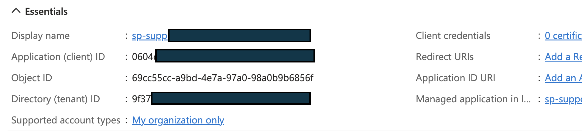
Generate an Azure Service Principal: Now this step is completely done in the Azure Portal (not Databricks workspace). Go to Azure Active Directory -> App Registrations -> Enter some Display Name -> Select “Accounts in this organisation only” -> Register. After the service principal is generated, you will need its Application (client) ID and Tenant ID as shown below:
Generate Client Secret and Grant access to Databricks API: We will need to create Client Secret and Register Databricks access. To generate client secret, remain on Service Principal’s blade -> Certificates & Secrets -> New Client secret -> Enter Description and Expiry -> Add. Copy and store the Client Secret’s Value (not ID) separately. Note: The client secret Value is only displayed once.
Further, In the API permissions -> Add a permission -> APIs my organization users tab -> AzureDatabricks -> Permissions.
Add SP to the workspace: Now, Databricks has the ability to sync all identities created to the workspace if “Identity Federation” is enabled. Unfortunately, for this customer this was not enabled. Next, they needed to assign permission for this SP. This step in done in your Databricks workspace. Go to Your Username -> Admin Settings -> Service Principals tab -> Add service principal -> Enter Application ID from the Step 1 and a name -> No other permissions required -> Add.
Get Service Principal Contributor Access: Once the service principal has been generated, you will need to get Contributor access to the subscription. You will need help of your Azure Admin for the same.
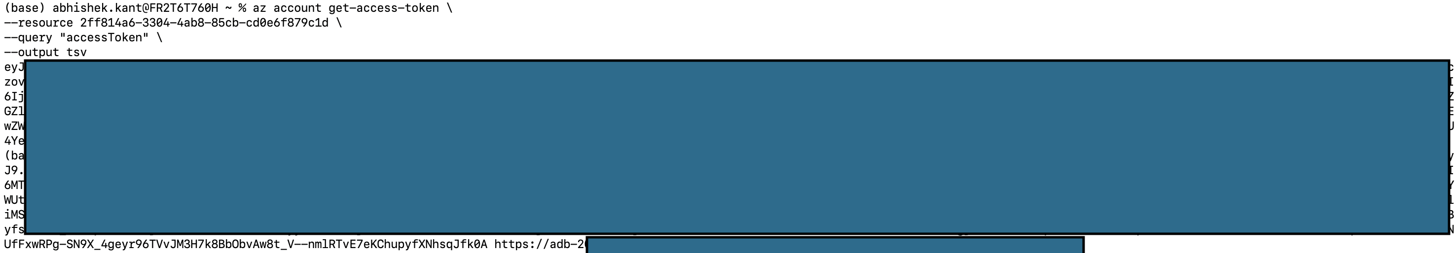
Authenticate as service principal: First login into Azure CLI as the Service Principal with the command:
The resource ID should be the same as shown above as it represents Azure Databricks.
This will create a Bearer token that you should preserve for the final step.
Assign permissions to SP to access Model Serving: The Model Serving endpoint has its own access control that provides for following permissions: Can View, Can Query, and Can Manage. Since we require to query the endpoint, we need to grant “Can Query” permission to the SP. This is done using the Databricks API endpoints as follows:
$ curl -n -v -X GET -H "Authorization: Bearer $ACCESS_TOKEN" https://$WORKSPACE_URL../api/2.0/serving-endpoints/$ENDPOINT_NAME

// $ENDPOINT_ID = the uuid field from the returned object
Replace @ACCESS_TOKEN with the bearer token generated in Step 6. The @WORKSPACE_URL should be replaced by the Databricks Workspace URL. Finally, the $ENDPOINT_NAME should be replaced by the name of the endpoint created.
This will give you the ID of the Endpoint as shown:
Next, you will need to issue the following command:
$ACCESS_TOKEN: From Step 6 $SP_NAME: Name of the service principal as created in Azure Portal $WORKSPACE_URL: Workspace URL @ENDPOINT_ID: Generated in the command above
Generate Databricks PAT from Azure AAD Token: While you have the Azure AAD token now available and it can used for calling the Model Serving endpoint, the Azure AAD tokens are shortlived. To create a Databricks PAT, you will need to make a POST request call to the following endpoint (I am using Postman for the request): https://$WORKSPAE_URL/api/2.0/token/create The Azure AAD Bearer token should be passed in the Authorization header. In the body of the request, just pass in a JSON with “comment” attribute. The response of the POST request will contain an attribute – “token_value” that can be used as Databricks PAT.
The token_value, starting with “dapi” is the PAT that can be used for calling the Model Serving Endpoint that is in a secure configuration using the Service Principal.
In the last post, we saw how we can use Pipelines to streamline our machine learning workflow.
We will start off with a fantastic feature that will blow the lid off your mind. All the effort done till now, in post I and II, can be done in 2 lines of code! Ah yes, this magic is possible with use of a feature called AutoML. Not only will it perform preprocessing steps automatically, it will also select the best algorithm from a multitude of them including XGBoost, LightGBM, Prophet etc. The hyper parameter search comes for free 🙂 If all this was not enough it will share the entire auto-generated code for your use and modification. So, the two magic lines are:
from databricks import automl
summary = automl.classify(train, target_col="category", timeout_minutes=20)
The AutoML requires you to specify the following:
Type of machine learning problem – Classification/ Regression/ Forecasting
Specify the training set, target column
Timeout after which the autoML will stop looking for better models.
While all this is very exciting, the real world use case of AutoML tends to be to create a baseline for model performance and give us a model to start with. In our case, the AutoML gave an RoC score of 91.8% (actually better than our manual work so far!!) for the best model.
Looking at the auto-generated Python notebook, here are the broad steps it took:
Load Data
Preprocessing
Impute values for missing numerical columns
Convert each categorical column into multiple binary columns through one-hot encoding
Train – Validation – Test Split
Train classification model
Inference
Determine Accuracy – Confusion matrix, ROC and Precision-Recall curves for validation data
This is broadly in line with what we did in our manual setup.
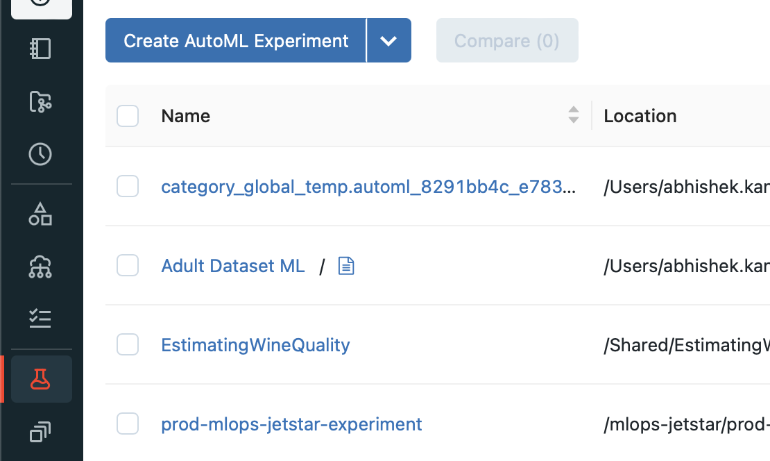
Apart from the coded approach we saw, you can create AutoML experiment using the UI from the Experiments -> Create AutoML Experiment button. If you can’t find the experiments tab, make sure that you have the Machine Learning persona selected in the Databricks workspace.
In an enterprise/ real world scenario, we will build many alternate models with different parameters and use the one with higest accuracy. Next, we deploy the model and use it for predictions with new data. Finally, the selected model will be updated over time as new data becomes available. Until now, we didn’t talk about how to handle these enterprise requirements or were doing it manually on best effort.
These requirements are covered under what we know as MLOps. Spark supports MLOps using an open source framework called MLFlow. MLFlow supports the following objects:
Projects: Provides a mechanism for storing machine learning code in a reusable and reproducible format.
Tracking: Allows for tracking your experiments and metrics. You can see the history of your model and its accuracy evolve over time. There is also a tracking UI available.
Model Registry: Allows for storing various models that you develop in a registry with an UI to explore the same. It also provides for model lineage (which MLflow experiment and run produced the model), stage transitions (for example from staging to production)
Model Serving: We can use serving to provide inference endpoints for either batch or inline processing. Mostly this will be made available as REST endopoints.
There is a very easy way to get started with MLFlow where we allow MLFlow to log automatically the metrics and models. This can be done using a single line:
import mlflow
mlflow.autolog()
This will log the parameters, metrics, models and the environment. The core concept to get with MLOps is the concept of runs. Each run is a unique combination of parameters and algorithm that you have executed. Many runs can be part of the same experiment.
To get started we can set name of the experiment with the command: mlflow_set_experiment(“name_of_the_experiment”)
To start tracking the experiments manually, we can setup the context as follows:
with mlflow.start_run(run_name="") as run:
   <pseudo code for running an experiment>
   mlflow.log_param("key","value")
   mlflow.log_metrics("key","value")
   mlflow.spark.log_model(model,"model name")
You can track parameters and metrics using log_param and log_metrics functions of mlflow object. The model can now be registered with the Model Registry using the function: mlflow.register_model(model_uri=””, name=””)
What is important here is the model_uri. The model_uri takes the form: runs:/<runid>/model. The runid identifies the specific run in the experiment and each model is stored at the model_uri location mentioned above.
You can now load the model and perform inference using the following code:
import mlflow

# Load model
loaded_model = mlflow.spark.load_model(model_uri)

# Perform inference via model.transform()
loaded_model.transform(data)
While we have seen how to track experiments explicitly, Databricks Workspaces also track the experiments automatically (from Databricks Runtime 10.3 ML and above). You can view the expriments and their runs in the UI via the Experiments sidebar of the Machine Learning persona.
You will need to click on the specific experiment (in our case Adult Dataset), that will show all the runs of the experiment. Click on the specific run to get more details about the run. The run will show the metrics recorded which is in our case was areaUnderRoC of 91.4%.
Under Artifacts, if you click on the model, you can see the URI of the model run. This URI can be used to register the model with the Model Registry and use it for predictions at any point in time.
MLFlow also supports indicating the state of the model for production. Different states supported by MLFlow are:
None
Staging
Production
Archived
Once your model is registered with the Model registry, you can change the state of the model to any other state with the function transition_model_version_stage() function.
From the model registry you are able to create model serving endpoint using the Serverless Real-Time Inference service that uses managed Databricks compute service to provide a REST endpoint.
In the earlier post, we went over some concepts regarding Machine Learning done with Spark ML. Here are primarily 2 types of objects relating to machine learning we saw:
Transformers: Objects that took a DataFrame, changed something in it and returned a DataFrame. The method used here was “transform”.
Estimator: Objects that are passed in a DataFrame and would apply an algorithm on it to return a transformer. E.g. GBTClassifier. We used the “fit” function to apply the algorithm on the Dataframe.
In our last example of predicting income level using Adult dataset, we had to change our input dataset to a format that is suitable for machine learning. There was a sequence of changes we had done e.g. converting categorical variables to numeric, One Hot Encoding & Assembling the columns in a single column. Everytime there is additional data available (which will be numerous times), we will need to do these steps again and again.
In this post, we will introduce a new Object that organises these steps in sequence that can be run as many times as needed and it is called the Pipeline. The Pipeline chains together various transformers and estimators in sequence. While we could do the machine learning without the Pipeline, it is a standard practice to put the sequence of steps in a Pipeline. Before we get there, let’s try to add an additional step in fixing our pipeline and that is to identify and remove Null data. This is indicated in our dataset as ‘?’.
To know how many null values exist let’s run this command:
from pyspark.sql.functions import isnull, when, count, col
adultDF.select([count(when(isnull(c), c)).alias(c) for c in adultDF.columns]).show()
The result shows that there are no null values. Inspecting the data, we see that null values have been replaced with “?”. We would need to remove these rows from our dataset. We can replace the ? with null values as follows:
adultDF = adultDF.replace('?', None)
Surprisingly this doesn’t change the ? values. It appeared that the ? is padded with some spaces. So we will use the when and trim function as follows:
from pyspark.sql.functions import isnull, when, count, col,trim
adultDF = adultDF.select([when(trim(col(c))=='?',None).otherwise(col(c)).alias(c) for c in adultDF.columns])
This replaces ? will null that we can now drop from our dataframe using dropna() function. The number of rows remaining are now 30,162.
Now let’s organise these steps in a Pipeline as follows:
from pyspark.ml import Pipeline

adultPipeline = Pipeline(stages = [wcindexer,eduindexer,maritalindexer,occupationindexer,relindexer,raceindexer,sexindexer,nativecountryindexer,categoryindexer,ohencoder,colvectors])
The stages list contains all the transformers we used to convert raw data into dataset ready for machine learning. This includes all the StringIndexers, OneHotEncoder and VectorAssembler. Next, the process of defining the GBTClassifier and BinaryClassificationEvaluator remains the same as in the earlier post. You can now include the GBTClassfier in the pipeline as well and run the fit() on this pipeline with train dataset as follows:
However, we can perform another optimization at this point. The model currently trained is based of a random split of values from the dataset. Cross Validation can help generalise the model even better by determining best parameters from a list of parameters and do it by creating more than one train and test datasets (called as folds). The list of parameters are supplied as ParamGrid as follows:
from pyspark.ml.tuning import CrossValidator, ParamGridBuilder

paramGrid = ParamGridBuilder()\
  .addGrid(gbtclassifier.maxDepth, [2, 5])\
  .addGrid(gbtclassifier.maxIter, [10, 100])\
  .build()

# Declare the CrossValidator, which performs the model tuning.
cv = CrossValidator(estimator=gbtclassifier, evaluator=eval, estimatorParamMaps=paramGrid)
The cross validator object takes the estimator, evaluator and the paramGrid objects. The pipeline will need to be modified to use this cross validator instead of the classifier object we used earlier as follows:
Machine Learning is most widely done using Python and scikit-learn toolkit. The biggest disadvantage of using this combination is the single machine limit that Python imposes on training the model. This limits the amount of data that can be used for training to the maximum memory on the computer.
Industrial/ enterprise datasets tend to be in terabytes and hence the need for a parallel processing framework that could handle enormous datasets was felt. This is where Spark comes in. Spark comes with a machine learning framework that can be executed in parallel during training using a framework called Spark ML. Spark ML is based on the same Dataframe API that is widely used within the Spark ecosystem. This requires minimal additional learning for preprocessing of raw data.
In this post, we will cover how to train a model using Spark ML.
In the next post, we will introduce the concept of Spark ML pipelines that allow us to process the data in a defined sequence.
The final post will cover MLOps capabilities that MLFlow framework provides for operationalising our machine learning models.
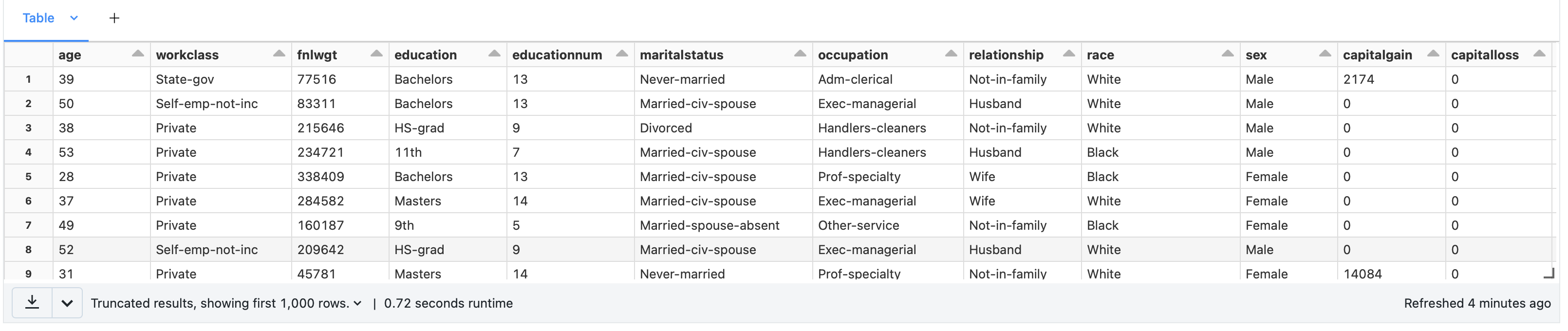
We are going to be Adult Dataset from UCI Machine Learning Repository. Go ahead and download the dataset from the “Data Folder” link on the page. The file you are interested to download is named “adult.data” and contains the actual data. Since the format of this dataset is CSV, I saved it on my local machine as adult.data.csv. The schema of this dataset is available in another file titled – adult.names. The schema of the dataset is as follows:
The prediction task is to determine whether a person makes over 50K in a year which is contained in the summary field. This field contains value of <50K or >=50K and is our target variable. The machine learning task is that of binary classification.
The first step was to upload the dataset from where it is accessible. I chose DBFS for ease of use and uploaded the file at the following location: /dbfs/FileStore/Abhishek-kant/adult_dataset.csv
Once loaded in DBFS, we need to access the same as a Dataframe. We will apply a schema while reading the data since the data doesn’t come with header values as indicated below:
We need to move towards making this dataset machine learning ready. Spark ML only works with numeric data. We have many text values in the dataframe that will need to be converted to numeric values.
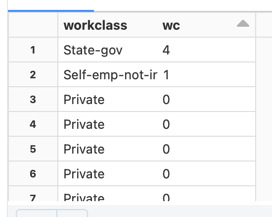
One of the key changes is to convert categorical variables expressed as string into labels expressed as string. This can be done using StringIndexer object (available in pyspark.ml.feature namespace) as illustrated below: eduindexer = StringIndexer(inputCol=”education”, outputCol =”edu”)
The inputCol indicates the column to be transformed and outputCol is the name of the column that will get added to the dataframe after converting to the categorical label. The result of the StringIndexer is shown to the right e.g. Private is converted to 0 while State-gov is converted to 4.
This conversion will need to be done for every column:
This creates what is called a “dense” matrix where a single column contains all the values. Further, we will need to convert this to “sparse” matrix where we have multiple columns for each value for a category and for each column we have a 0 or 1. This conversion can be done using the OneHotEncoder object (available in pyspark.ml.feature namespace) as shown below: ohencoder = OneHotEncoder(inputCols=[“wc”], outputCols=[“v_wc”])
The inputCols is a list of columns that need to be “sparsed” and outputCols is the new column name. The confusion sometimes is around fitting sparse matrix in a single column. OneHotEncoder uses a schema based approach to fit this in a single column as shown to the left.
Note that we will not sparse the target variable i.e. “summary”.
The final step for preparing our data for machine learning is to “vectorise” it. Unlike most machine learning frameworks that take a matrix for training, Spark ML requires all feature columns to be passed in as a single vector of columns. This is achieved using VectorAssembler object (available in pyspark.ml.feature namespace) as shown below:
As you can see above, we are adding all columns in a vector called as “features”. With this our dataframe is ready for machine learning task.
We will proceed to split the dataframe in training and test data set using randomSplit function of dataframe as shown:
(train, test) = adultMLDF.randomSplit([0.7,0.3])
This will split our dataframe into train and test dataframe in 70:30 ratio. The classifier used will be Gradient Boosting classifier available as GBTClassifier object and initialised as follows:
from pyspark.ml.classification import GBTClassifier

classifier = GBTClassifier(labelCol="catlabel", featuresCol="features")
The target variable and features vector column is passed as attributes to the object. Once the classifier object is initialised we can use it to train our model using the “fit” method and passing the training dataset as an attribute:
gbmodel = classifier.fit(train)
Once the training is done, you can get predictions on the test dataset using the “transform” method of the model with test dataset passed in as attribute:
adultTestDF = gbmodel.transform(test)
The result of this function is addition of three columns to the dataset as shown below:
A very important task in machine learning is to determine the efficacy of the model. To evaluate how the model performed, we can use the BinaryClassificationEvaluator object as follows:
In the initialisation of the BinaryClassificationEvaluator, the labelCol attribute specifies the actual value and rawPredictionCol represents the predicted value stored in the column – rawPrediction. The evaluate function will give the accuracy of the prediction in the test dataset represented as AreaUnderROC metric for classification tasks.
You would definitely want to save the trained model for use later by simply saving the model as follows:
gbmodel.save(path)
You can later retrieve this model using “load” function of the specific classifier:
from pyspark.ml.classification import GBTClassificationModel
classifierModel = GBTClassificationModel.load(path)
You can now use this classification model for inferencing as required.
A customer wanted to know the total cost of running Azure Databricks for them. They couldn’t understand what DBU (Databricks Units) was, given that is the pricing unit for Azure Databricks.
I will attempt to clarify DBU in this post.
DBU is just really an abstraction not related to any amount of compute or compute metrics. At the same time, it changes with the following factors:
When there is a change in the kind of machine you are running the cluster on
When there is change in the kind of workload (e.g. Jobs, All Purpose)
The tier / capabilities of the workload (Standard / Premium)
The kind of runtime (e.g. with or without Photon)
So, the DBUs really measure the consumption of resources. It is billed on a per second basis. The monetary value of these DBUs is called $DBU and is determined by a $ rate charged per DBU. Pricing rate per DBU is available here.
You are paying DBUs for the software that Databricks has made available for processing your Big Data workload. The hardware component needed to run the cluster is charged directly by Azure.
When you visit the Azure Pricing Calculator and look at the pricing for Azure Databricks, you would see that there are two distinct sections – one for compute and another for Databricks DBUs that specifies this rate.
The total price of running an Azure Databricks cluster is a combination of the above two sections.
Let us now understand if we are running a cluster of 6 machines what is the total cost likely to be:
For the All Purpose Compute running in West US in Standard tier with D3 v2, the total cost for compute (in PAYG model) is likely to be USD 1,222/ month.
From the calculator you can see that DBU consumption is 0.75 DBU with a rate of USD 0.4/ hr. So, the total cost of running 6 D3 v2 machines in the cluster will be $ 219 * 6 = $ 1,314.
The total cost hence would be USD 2,536.
From an optimization perspective, you can reduce your hardware compute by making reservations e.g. 1 yr or 3 yrs in Azure. DBUs from the Azure calculator doesn’t have any upfront commitment discounts available. However, they are available if you contact Databricks and request for discount on a fixed commitment.
Spark provides a lot of connectors to load data from various formats. Whether it is a CSV or JSON or Parquet you can use the magic of “spark.read”.
However, there are times when you would like to create a DataFrame dynamically using code. The one use case that I was presented with was to create a dataframe out of a very twisted incoming JSON from an API. So, I decided to parse the JSON manually and create a dataframe.
The approach we are going to use is to create a list of structured Row types and we are using PySpark for the task. The steps are as follows:
Define the custom row class
personRow = Row("name","age")
2. Create an empty list to populate later
community = []
3. Create row objects with the specific data in them. In my case, this data is coming from the response that we get from calling the API.
qr = personRow(name, age)
4. Append the row objects to the list. In our program, we are using a loop to append multiple Row objects to the list.
In this tutorial we are implementing Microsoft Azure Ad Login in React single-page app and retrieve user information using @azure/msal-browser.
The MSAL library for JavaScript enables client-side JavaScript applications to authenticate users using Azure AD work and school accounts (AAD), Microsoft personal accounts (MSA) and social identity providers like Facebook, Google, LinkedIn, Microsoft accounts, etc. through Azure AD B2C service. It also enables your app to get tokens to access Microsoft Cloud services such as Microsoft Graph.
In the below App.js file code we are using Context and Reducer for managing the login state. useReducer allows functional components in React access to reducer functions from your state management
First we initialize the initial values for reducer, Reducers are functions that take the current state and an action as arguments, and return a new state result. In other words, (state, action) => newState
You can see the code form 17 line where we created reducer with using switch case “LOGIN” and “LOGOUT”. and from Line 58 we use the context that defined in line 6 and passing the reducer values to it.
And In a line 66 : we are checking the state.isAuthenticated or not , if it’s not the page redirect to the home page and if it’s Authenticated it will be redirected to the admin dashboard home page.
Now we are coming the the Login Component with Azure Ad using with @azure/msal-browser
In a below code we are importing AuthContext from App.js and PublicClientApplication from @azure/msal-browser.
and In a 7th line we created constant variable “dispatch” with providing the reference of AuthContext then we created the msalInstandce variable using the PublicClientApplication and providing the clientId, authority and redirectUri in auth block.
In a line 22 we created the startlogin function then we created the loginRequest variable and providing the scope for login.
and In a line 31 we use the msalInstance.loginPopup(loginRequest) for getting pop up window for login and in a “loginRespone” variable save the login response. then we are fetching the username and token form loginRespone. dispatch to the AuthContext (see line 41).
And In a line 56 we created a button it’s call the startLogin function on click event.
One of our customers had a requirement of copying data that was locked in an Azure Databricks Table in a specific region (let’s say this is eastus region). The tables were NOT configured as Delta tables in the originating region and a subset of personnel had access to both the regions.
However, the analysts were using another region (let’s say this is westus region) as it was properly configured with appropriate permissions. The requirement was to copy the Azure Databricks Table from eastus region to westus region. After a little exploration, we couldn’t find a direct/ simple solution to copy data from one Databricks region to another.
One of the first thoughts that we had was to use Azure Data Factory with the Databricks Delta connector. This would be the simplest as we would simply need a Copy Data activity in the pipeline with two linked services. The source would be a Delta Lake linked service to eastus tables and the sink would be another Delta Lake linked service to westus table. This solution faced two practical issues:
The source table was not a Delta table. This prevented the use of Delta Lake linked service as source.
When sink for copy activity is a not a blob or ADLS, it requires us to use a staging storage blob. While we were able to link a staging storage blob, the connection could not be established due to authentication errors during execution. The pipeline error looked like the following:
Operation on target moveBlobToADB failed: ErrorCode=AzureDatabricksCommandError,Hit an error when running the command in Azure Databricks. Error details: shaded.databricks.org.apache.hadoop.fs.azure.AzureException: shaded.databricks.org.apache.hadoop.fs.azure.AzureException: Unable to access container adf-staging in account xxx.blob.core.windows.net using anonymous credentials, and no credentials found for them in the configuration. Caused by: shaded.databricks.org.apache.hadoop.fs.azure.AzureException: Unable to access container adf-staging in account xxx.blob.core.windows.net using anonymous credentials, and no credentials found for them in the configuration. Caused by: hadoop_azure_shaded.com.microsoft.azure.storage.StorageException: Public access is not permitted on this storage account..
On digging deeper, this requirement is documented as a prerequisite. We wanted to use the Access Key method but it requires the keys to be added into Azure Databricks cluster configuration. We didn’t have access to modify the ADB cluster configuration.
To work with this, we found the following alternatives:
Use Databricks notebook to read data from non-Delta Tables in Databricks. The data can be stored in a staging Blob Storage.
To upload the data into the destination table, we will again need to use a Databricks notebook as we are not able to modify the cluster configuration.
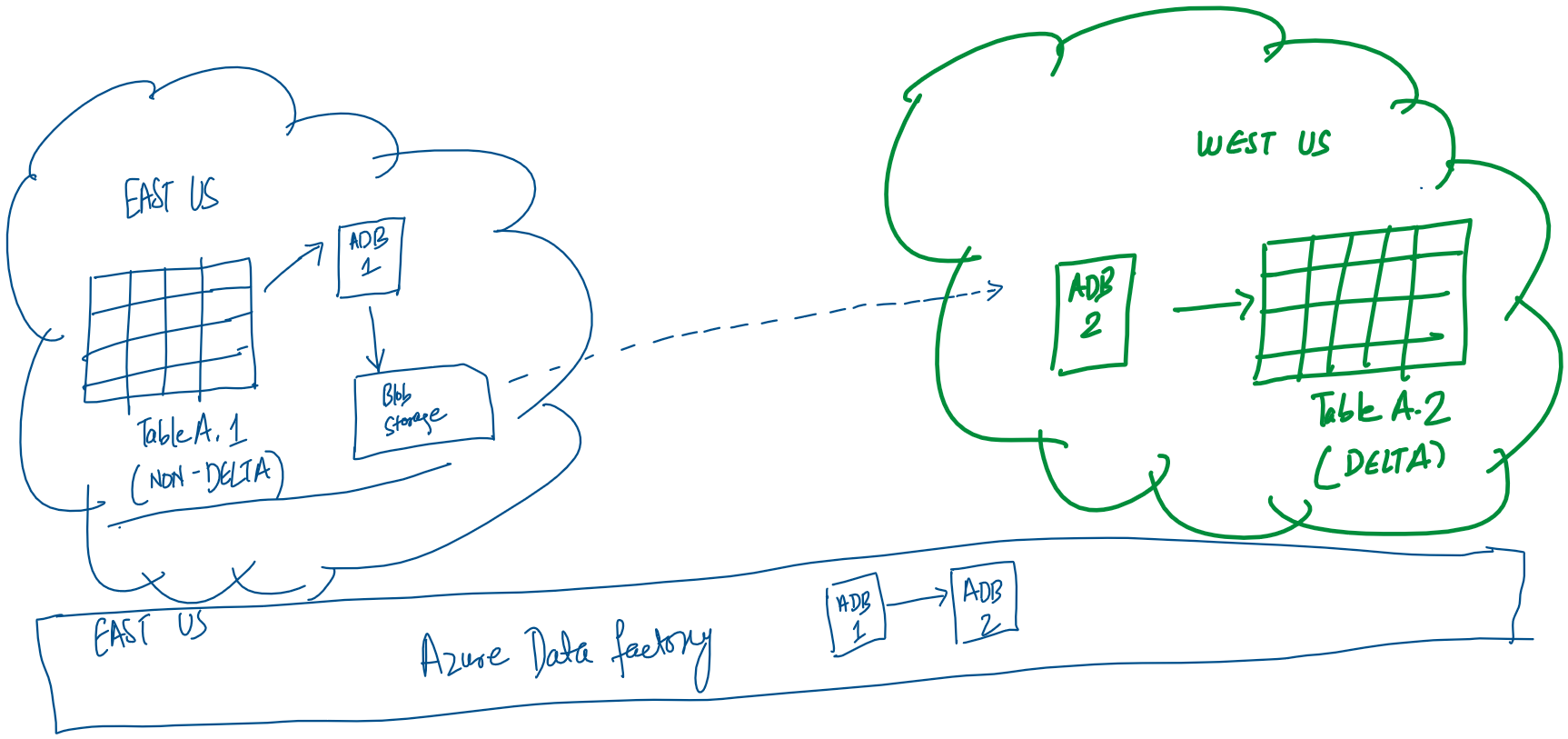
Here is the solution we came up with:
In this architecture, the ADB 1 notebook is reading data from Databricks Table A.1 and storing it in the staging blob storage in the parquet format. Only specific users are allowed to access eastus data tables, so the notebook has to be run in their account. The linked service configuration of the Azure Databricks notebook requires us to manually specify: workspace URL, cluster ID and personal access token. All the data transfer is in the same region so no bandwidth charges accrue.
Next the Databricks ADB 2 notebook is accesses the parquet file in the blob storage and loads the data in the Databricks Delta Table A.2.
The above sequence is managed by the Azure Data Factory and we are using Run ID as filenames (declared as parameters) on the storage account. This pipeline is configured to be run daily.
The daily run of the pipeline would lead to a lot of data in the Azure Storage blob as we don’t have any step that cleans up the staging files. We have used the Azure Storage Blob lifecycle management to delete all files not modified for 15 days to be deleted automatically.
The next step to building an API is to protect it from anonymous users. Azure Active Directory (AD) serves as an identity platform that can be used to secure our APIs from anonymous users. After the authentication is enabled, users will need to provide a OAuth 2.0/ JST token to gain access to our API.
Let us begin to implement Azure AD Authentication in ASP.NET Core 5.0 Web API.
I will be creating ASP.NET Core 5.0 project and show you step by step how to enable authentication on it using Azure AD Authentication. We will be doing it using the MSAL package from nuget.
Prerequisites
Before you start to follow steps given in this article, you will need an Azure Account, and Visual Studio 2019 with .NET 5.0 development environment step.
Creating ASP.NET Core 5.0 web application
Open visual studio and click on Create a new project in the right and select “Asp.net core web app” as shown in below image and click next.
In the configure your new project section enter name and location of your project as shown in below image and click next
In the additional information step, select .NET 5.0 in the target framework, Authentication Type to none and check Configure HTTPS checkbox and click on create.
Configuring ASP.NET Core 5.0 App for Azure AD Authentication
Open appsettings.json of your web api and add following lines of code.
Next, in the Startup.cs, go to Configure method and add app.UseAuthentication(); line before app.UseAuthorization(); line.
Next, open any Controller and add [Authorize] attribute:
    [Authorize]
    [Route("[controller]")]
    [ApiController]
    public class SupportController : ControllerBase
    {

    }
Save all files and run your project.
You will notice that once you run the project, and try to access any method in support controller from the browser you will get return the HTTP ERROR 401 ( Unauthorized client error).
Conclusion
Our API is no longer available for anonymous access. It is now protected by Azure AD Authentication.
The legacy SOAP based web services/ APIs are still in use at a lot of organisations. While Telerik Test Studio has direct support for REST based APIs, testing SOAP web services requires a few additional steps.
In the short video below, we share how we can test SOAP based APIs in Test Studio:
The three things needed include:
A Test Oracle to encapsulate web services call: Built easily with Visual Studio
Coded Steps in Test Studio
Data Driven tests for testing various inputs
The transcript of the video is as follows:
Can Test studio test APIs? And i think most of you know the answer that it does support testing REST APIs. Recently one of the customers asked me if Telerik Test Studio can be used for automation of SOAP-based web services and the answer to that is it can be done in telerik test studio using coded tests.
In this video we will see how we can test SOAP based web services using Test Studio. The soap web service that i am using for testing is a publicly available service that converts digits to numbers. So in this web service i’m going to use the number and what it allows me to do is enter a number so let’s enter 789 and by invoking this i get the the words or the digits converted into words as seven eighty nine. So this is the web service that i’m going to test back in the test studio.
I have authored a test that will feed in various digits and verify if the web service returns the correct words for those digits. For the same i have put in some local data with digits in one column and in words in the second column. So this is going to be a data driven test. Let’s test this with our script. I’m just starting the test with the headless chrome as execution engine because web services don’t have a UI. The test has started and you can see that i’ve got the debugger going and already the test has finished.
Now there were four iterations of this test, this being a data driven test and if you want to see the logs for each of the iterations that’s visible here as well. In iteration number one you will notice the overall result is pass. In fact here it shows we’re using chrome headless version and our test was successful in iteration number two where we had put in two three eight nine the result is fail and the failure information is also mentioned here. Well we were expecting the web service to return two hundred and eighty nine but the web service actually returned two thousand three hundred and eight nine not eighty nine. So this actually indicates a failure on the assertion. Well the test continued because we have marked this step as continue on failure. Iteration number three has result as pass wherein we passed in a single digit 4 and we also got back the same value which is four. Iteration or the last iteration here is checking for digits 10 and inwords it should also be ten and once again the overall result is pass. So here you can see its result is pass but your overall result is a fail because one of the iterations here did actually fail.
So in the next few minutes we will see how we had created this SOAP test in telerik test studio. So to work the magic of a soap api test and it’s actually quite painless in telerik test studio. You need three things:
1. the first is a test oracle number
2. two is the coded step in test studio and
3. number three is data driving the verification
Okay let’s start with the test oracle. The test oracle is an external assembly that you are going to use within test studio inside your script but this assembly is going to be created by someone else. So what i had gotten done was to call the SOAP API using a visual studio function of adding web service reference and created that project as an assembly. Now the next step would be to add that assembly in test studio so if you go to your project and go to settings you will have a section that says script. Now within this section you will notice some assemblies that are automatically referenced here. Now if you notice this reference, this is something that has been added as a custom reference and this is where my test oracle has been created. So this assembly uses a simple function to invoke the SOAP API and provides a simple programmatic interface to invoke this soap service. So if you want to add more test oracles or external assemblies you can click on add reference and that’s what allows you to refer any .NET based assembly. So that takes care of the first step which is of getting a test article in place.
The second step is to add a coded step in my test script so you can add a coded step in test studio by using the step builder. Here where i’ve selected the common and within it there is a coded step and i can click on add step button. And this will add a coded step so that’s already done here. As you can see the coded step i am using is titled sample soap underscore coded step. In fact the code for this is available in the cs file located here. I just opened up the cs file the first thing that i need to do is to add a reference or to soap call namespace now in my function which is called as sample code underscore coded step. I am creating an instance of the object and within this i am passing in the specific digits. And finally i’m asserting if the digit that i have passed is the same as the one it should be in words.
Now the syntax here is slightly different. The syntax looks different because we are actually doing the third step in this demo which is data driving the verification. To data drive the verification as well as input values you’ve got to use the data and the specific column that you have created. So that’s what i’m using, so data and digits. And since the function towords requires me to give in an integer value i’m passing that in to the towords function of the test oracle. So conversion service and the function towords are actually coming from the test oracle. Finally i’m adding an assertion to see if the value that has been returned which is the nword value here and then the value that is there in my data driven column which is called inwords is also mentioned here. So both of them need to match up for this test to succeed. To quickly check where we had put in this data driven values we can go back to the test script and down below next to the test steps you will find the local data tab. And that’s where we can manually add these values.
This demonstration has showed you that Test Studio can be easily used to data drive SOAP based APIs automation
Enjoy watching the video and share your questions in the comments section below.
We got a request from our customer wanting to use a CSV file as Data Source in Telerik Report Designer to generate the report. They were unable to parse DateTime column to DateTime data type in Telerik Report Designer because the CSV returns the column with double quotes for example (“4/14/2021 12:42:25PM”).
Values can be easily cast to DateTime in Telerik Reporting during the datasource definition. The issue here was the quotes that came in the datasource.
In this blog post, we will explore how we can work with this scenario using Expressions provided by Telerik Report Designer..
First, we need to Add Data Source so click on Data in Menu then select the CSV Data Source and select and then click on Next button as below :
check the checkbox if CSV file has headers then click on NEXT button.
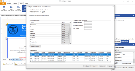
Now we the screen appear for Map columns to type and you can see the StartTime column below with double quotes:
Now we try to change the type of StartTime column string to DateTime. Now need to provide Date format in our case like yyyy-mm-dd hh:ss but in our case it will not work and the column will show blank.
Cause of blank again we need the change DateTime to String and Click on NEXT Button and Finish.
Now to the Data Source is connected with the report. the customer want the report with the parameter of data. So we need to convert StartTime(string) to StartTime(DateTime) using expression.
First we need to remove double quotes from StartTime using Replace function.
//Syntax of Replace function
=Replace(text, old substirng, new substring)

In a below code we take a text from Fields.StartTime and provide old substring that to be remove is double quotes in single quotes. and new substring is blank.

=Replace(Fields.StartTime,'"',"")
We got a StartTime in string without double quotes. so now we need to convert String to DateTime using CDate(value)Funciton. In a CDate function we provide the above Replace function that returning the StartTime without double qoutes.
= CDate(Replace(Fields.StartTime,'"',""))
Now we got the StartTime with the type of DateTime. and the above Expression we can use any where we want like filter the data and making parameter range with StartTime.
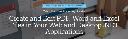
We get frequent requests from customers wanting to build a document using a template with header and footer and just including text in the Word document using ASP.NET Core.
We can achieve this using the TelerikWordsProcessing library. In this blog post, we will explore how.
You can do this by importing the document template with the DocxFormatProvider (if the template is a DOCX document or with any other of the supported by the WordsProcessing format providers) into a RadFlowDocument, edit its content using the RadFlowDocumentEditor and export it with the appropriate format provider.
First, you need to to install Telerik.Documents.Flow NuGet package see below picture where I am using Trial version of Telerik.
Add Template.docx file in root directory with header and footer.
In Program.cs file
Step 1 : Add below mentioned namespaces :
using System.Diagnostics;
using Telerik.Windows.Documents.Flow.FormatProviders.Docx;
using Telerik.Windows.Documents.Flow.Model;
using Telerik.Windows.Documents.Flow.Model.Editing;
Step 2 : Create RadFlowDocument object.
RadFlowDocument document;
Step 3 : And add the DocxFormatProvider for importing the DOCX Template in RadFlowDocument object “document”.
DocxFormatProvider provider = new DocxFormatProvider();

string templatePath = "Template.docx";

  using (Stream input = File.OpenRead(templatePath))
   {
       document = provider.Import(input);
   }
Step 4 : Now add the RadFlowDocumentEditor for editing the RadFlowDocument with providing it’s object. and with the RadFlowDocumentEditor object “editor” we are inserting the text.
RadFlowDocumentEditor editor = new RadFlowDocumentEditor(document);
editor.InsertText("Telerik WordsProcessing Library");
Step 5 : Now Define the Output of Document path. and export the document using above mentioned RadFlowDocumentEditor object “provider”.


 Save and exit.


 The Indian government has recently passed the
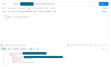


 This would be the simplest as we would simply need a Copy Data activity in the pipeline with two linked services. The source would be a Delta Lake linked service to eastus tables and the sink would be another Delta Lake linked service to westus table. This solution faced two practical issues: